Explainability
Data generators generate geodata from a preference model an/or a particular geometry computation. They are able to decompose a specific result and explain you where it comes from.
This information is retrieved for you and available in the explanation tab of the data analysis menu, whenever you are checking the result of a DataGenerator in a project. Then you click on a geometry feature on the map to see its explanations.
Note
If this tab is available for all project data generators, only the preference model itself is explainable.
Note
Only uptodate data have explanation, outdated data must be reprocessed in order to view its explanation.
There are two types of processing models:
preference models: computes result based on prefernces modelling
geometric models: modifies geometries/features of the data, potentially aggregating multiple input features together
Preference Models
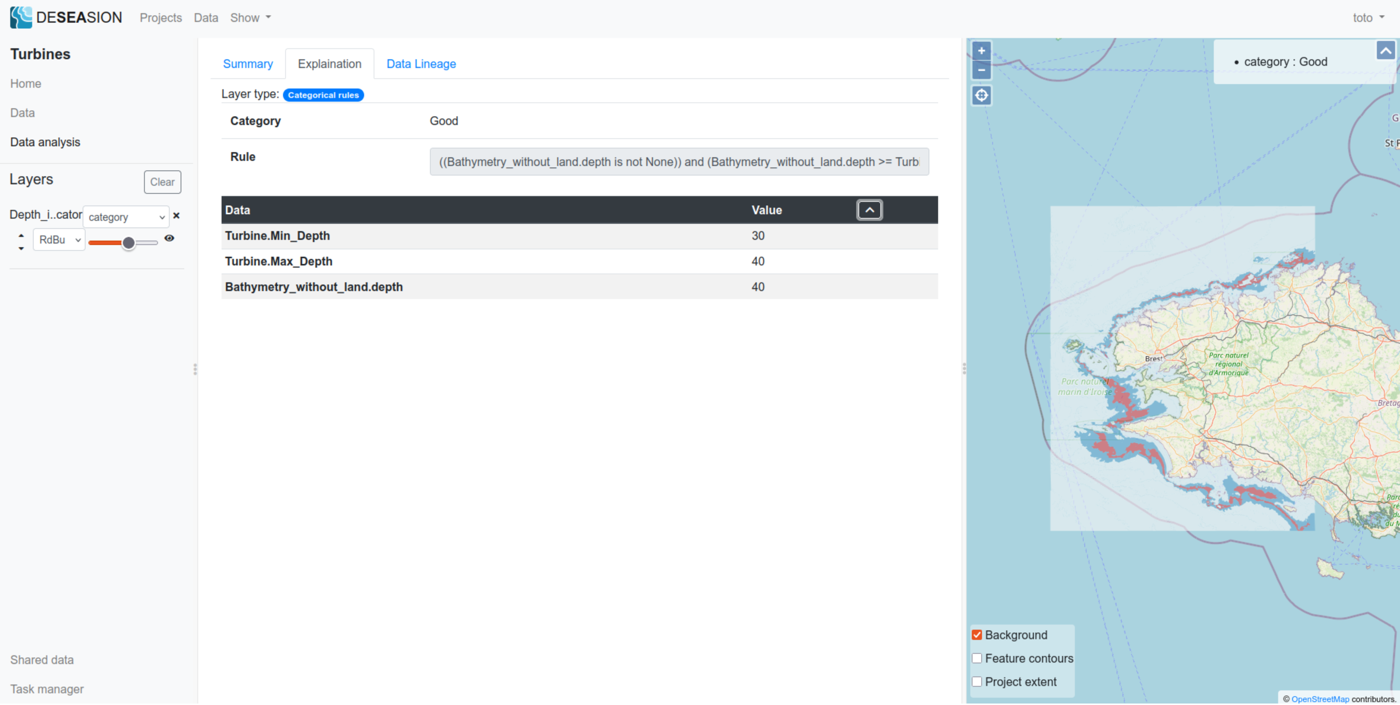
Categorical rules
The “categorical rules” preference model displays the following information in its explanation tab:
Category: the category resulting from the computation (i.e. the output)
Rule: the category rule that got activated and thus explains the result (the first activated one)
Data tab: shows the input value for this feature used to compute its category
Below a screenshot showing an example:
MR-Sort
MR-Sort displays the following information in its explanation tab:
Data comparison with its category bounding profiles: a plot showing the values of the feature for each input attribute, compared to the bounding profiles (note: higher is better, missing values for the data are not represented)
Profile cumulated weights comparison: a plot showing for each profile, the stacked attribute weights (added whenever the feature input is better or equal to the profile on this attribute), and the threshold used to rank the feature as better than the profile
Data tab: shows the input value for this feature used to compute its category
Please find in the following 2 screenshots an example, where the feature compares thusly with the profiles:
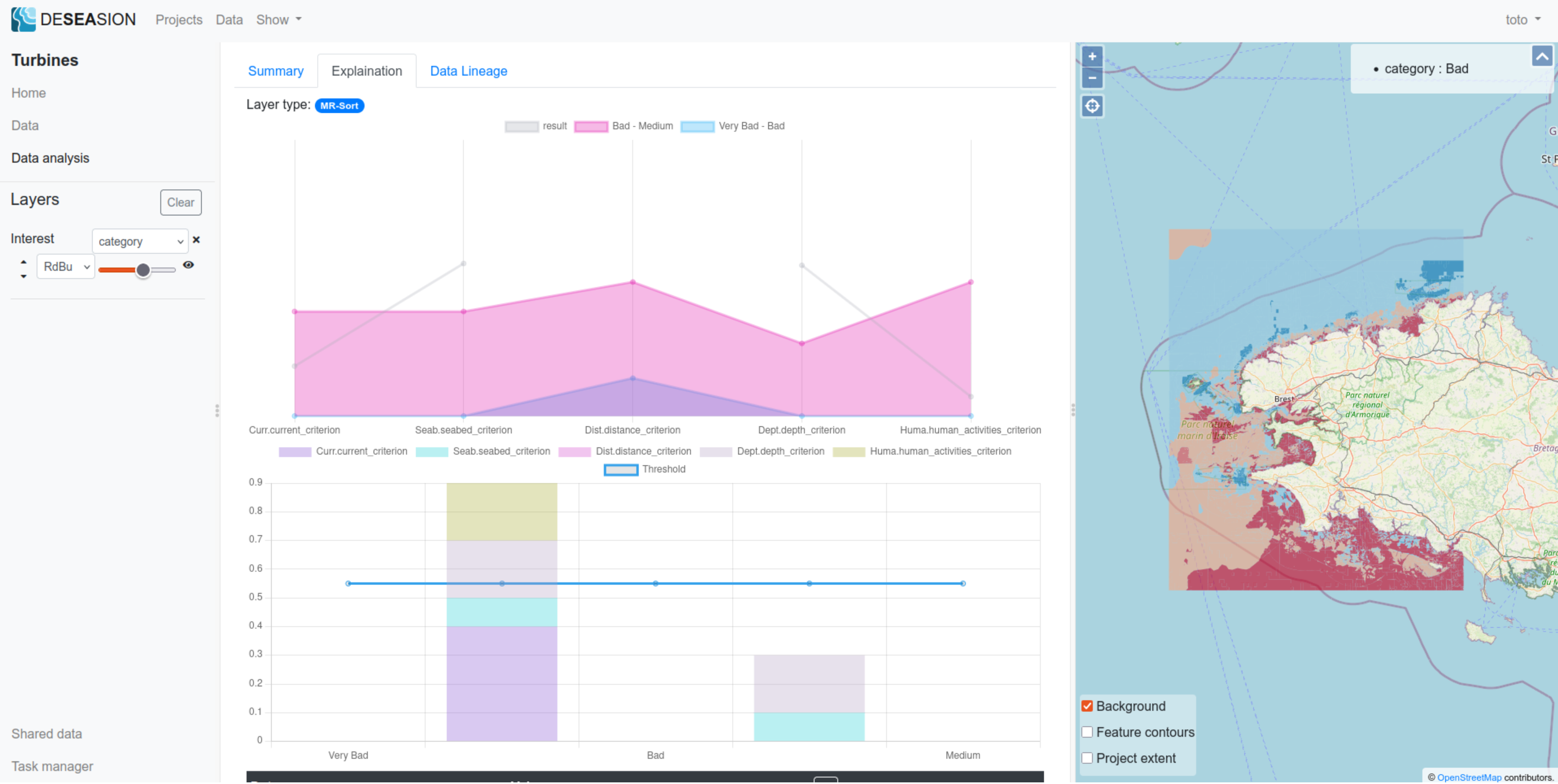
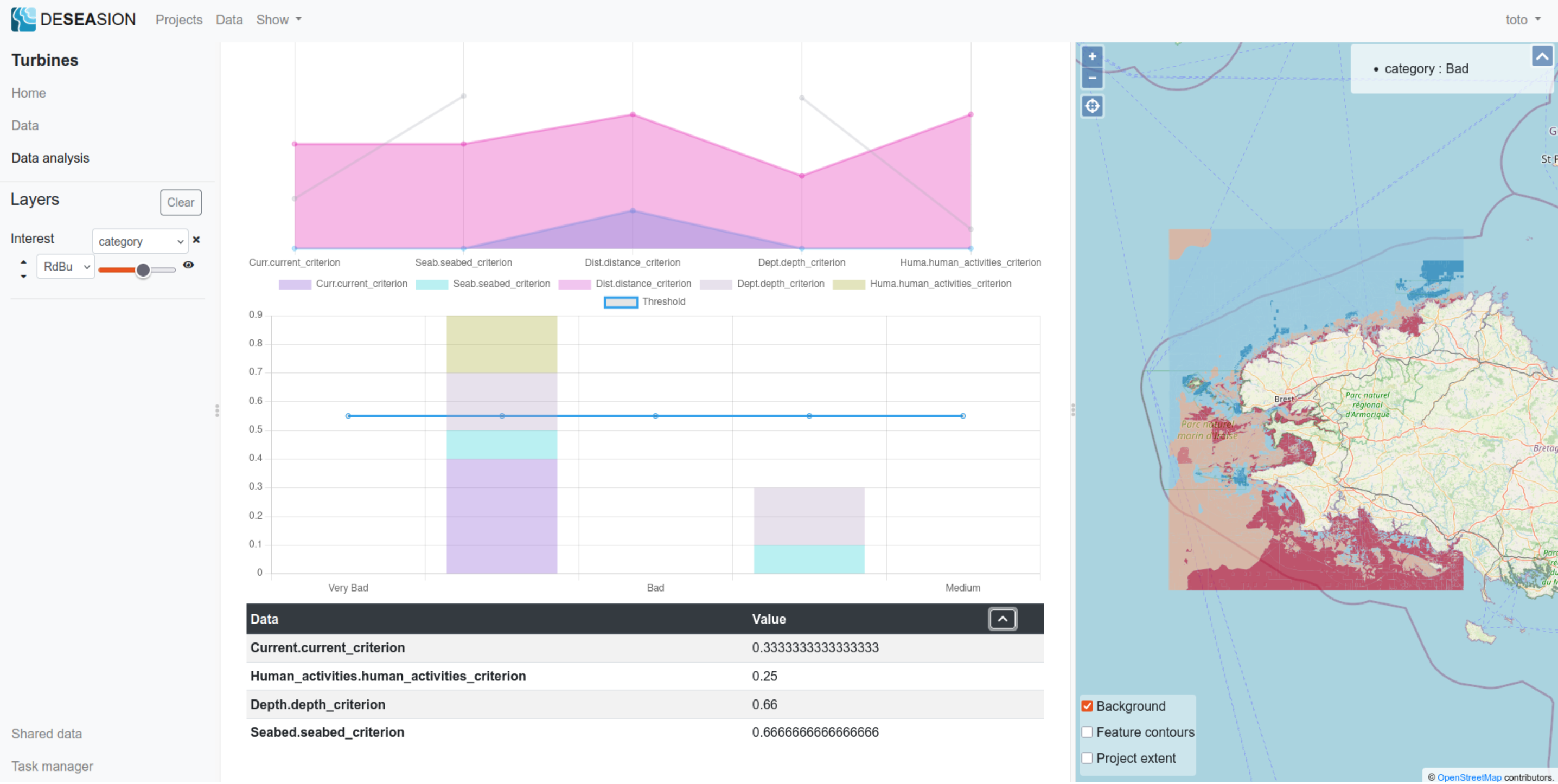
Between the lower (Very Bad - Bad) and upper (bad - Medium) profiles on the Current.current_criterion and Human_activities..human_activities_criterion attributes: therefore contributing their weights for the comparison with the lower profile
Better than both profiles on the Seabed.seabed_criterion and Depth.depth_criterion attributes: therefore contributing their weights for both profile comparisons
Missing value for Distance.distance_criterion attribute: thus considered worst than both and not adding its weight
The cumulated weights (0.9) for the comparison with the lower (Very Bad - Bad) profile is higher than the model threshold (0.55), thus the feature is better than this profile. The cumulated weights fell short (0.3) for the comparison with the upper profile (Bad - Medium), thus the feature is worst than it. This explains the final category (Bad) returned by the MR-Sort model.
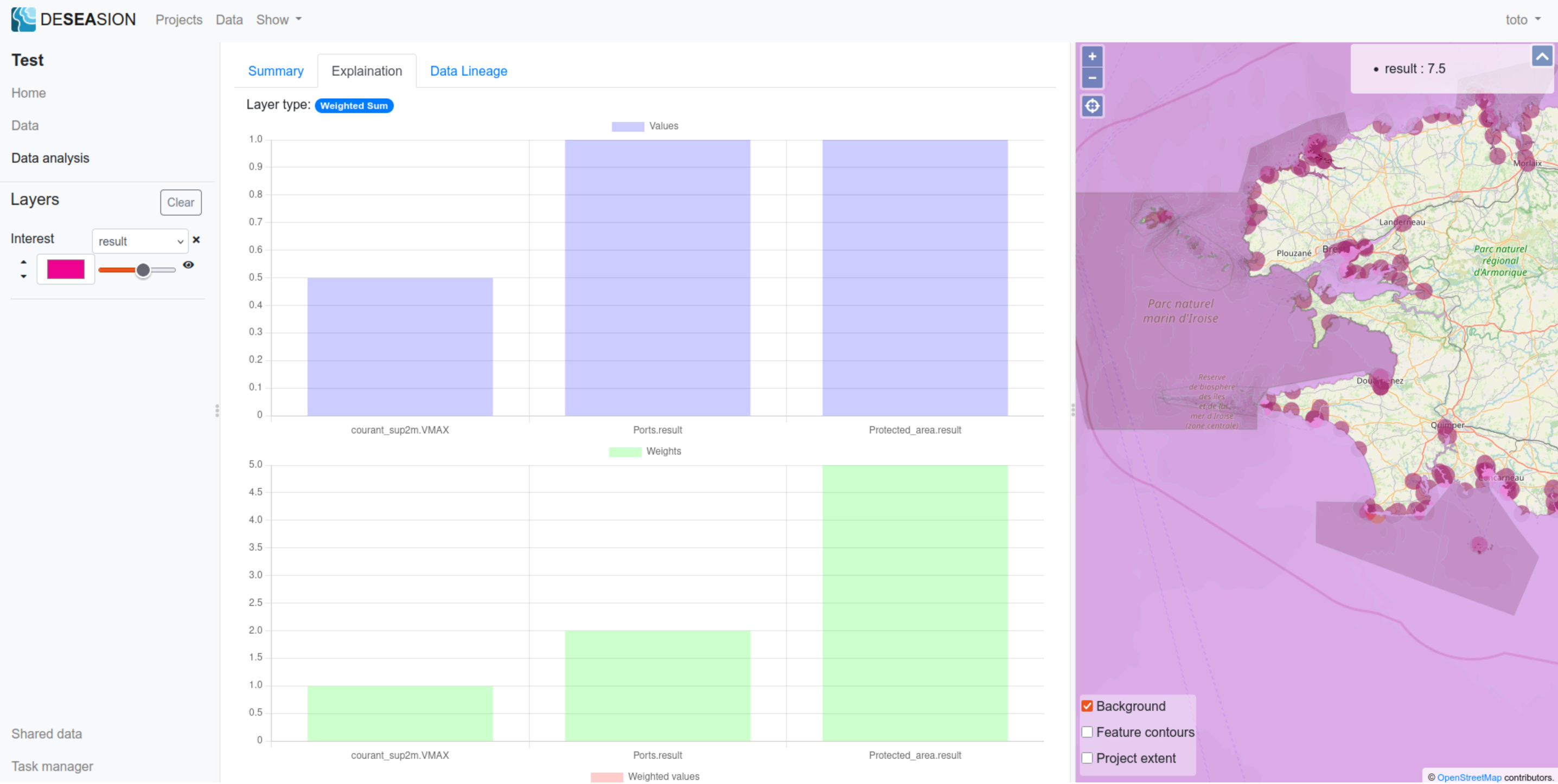
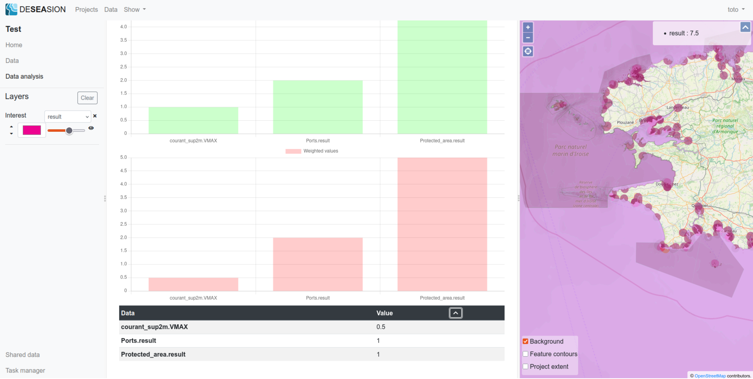
Weighted Sum
The weighted sum shows the following information in its explanation tab:
Raw input values of the feature
Weights per attributes
Weighted input values for the feature (value multiplied by the corresponding weight for each attribute)
Data tab: shows the input value for this feature used to compute its result value
Please find the screenshots showing an example of such explanation:
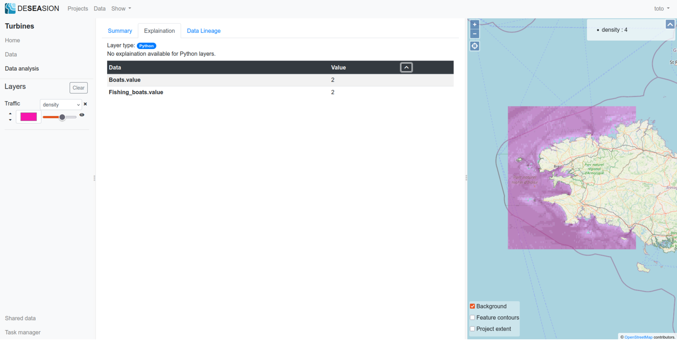
Python
The python model does not have a computed explanation, as it uses user-supplied arbitrary code. It does show the feature input values though.
Geometric Models
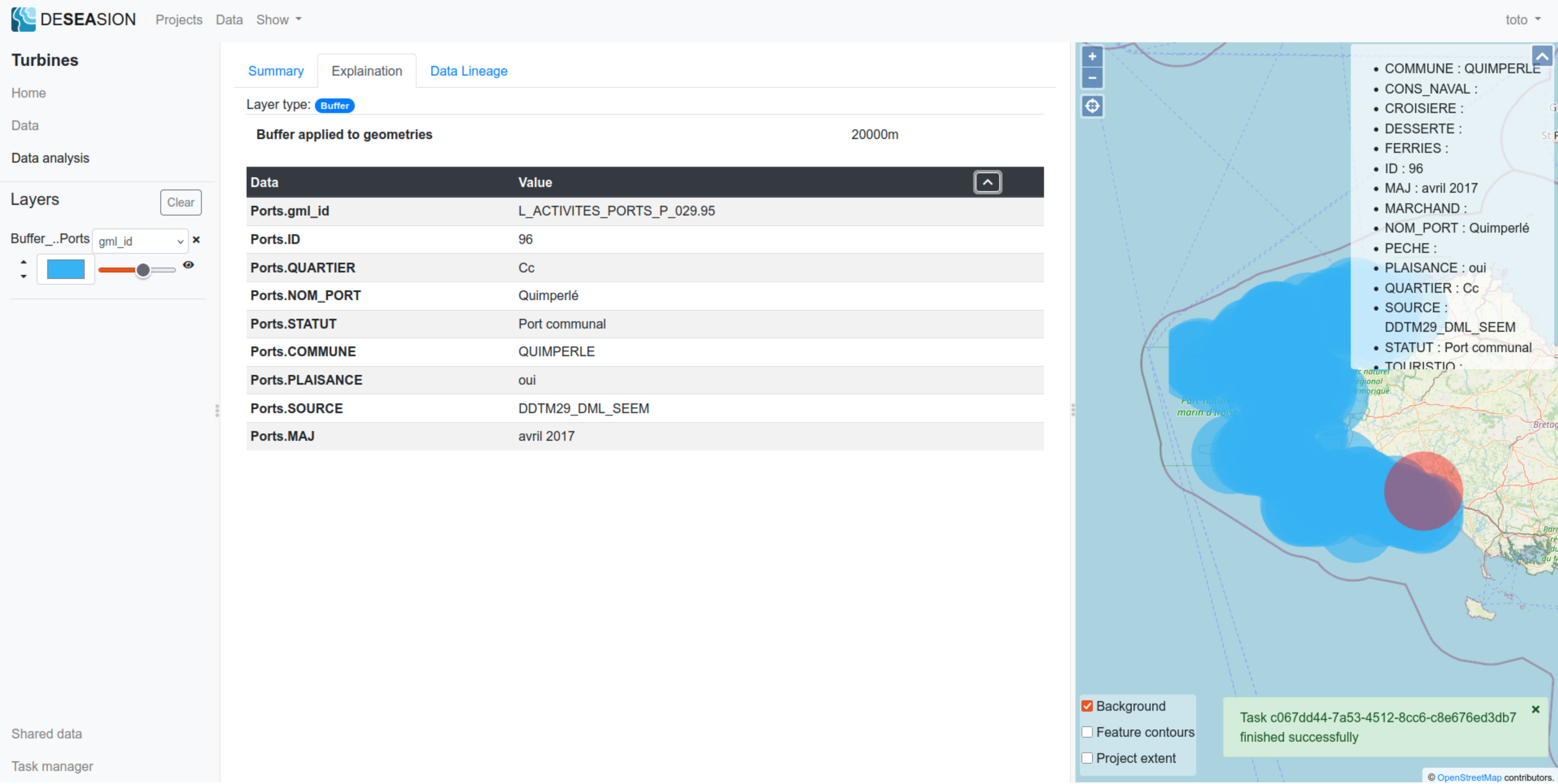
Buffer
The buffer shows the following information in its exlanation tab:
Buffer width: indicates the width of the buffer applied to the input layer
Data tab: shows the values for this feature, directly taken from its input
Below a screenshot showing an example:
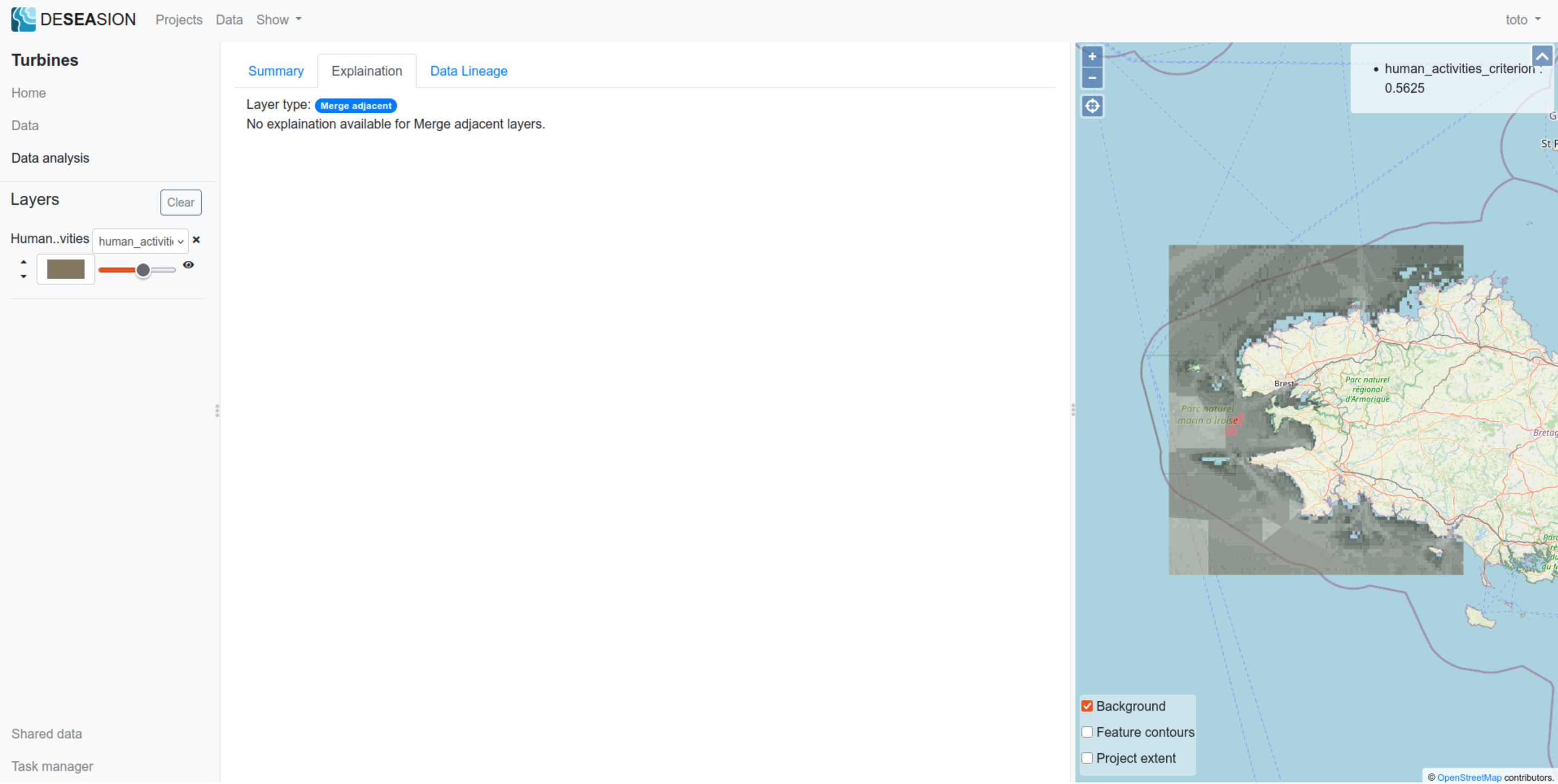
Merge Adjacent
This “Merge Adjacent” model squashes multiple jointed geometries sharing the same values. Therefore it does not have a particular explanation (result values is the shared input values).
Below a screenshot showing an example:
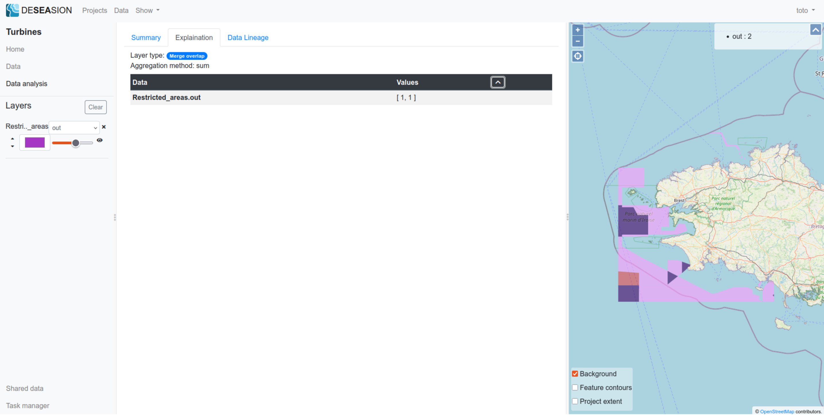
Merge Overlap
This “Merge Overlap” model aggregates multiple overlapping geometries into one. It shows the folowing explanation:
Aggregation method: method used to aggregate every value (per attribute) of its input geometries
Data tab: shows for each attribute, the values of each overlapping input features (i.e the values aggregated by this model)